DatasetMIRACLE

DatasetMIRACLE is an experimental (semi-synthetic) microphone array data generator that builds multi-source source cases by convolving synthetic source signals with measured spatial room impulse responses (SRIRs) from the MIRACLE dataset. The workflow is analogous to DatasetSynthetic, but the propagation operator is given by measured SRIRs instead of an analytic free-field model.

Multi-source scenes are realized by superposition of individually convolved source signals. By default, AcouPipe follows the same statistical scene model as in the synthetic generator (Poisson-distributed number of sources, normally distributed source positions, Rayleigh- distributed source strengths).

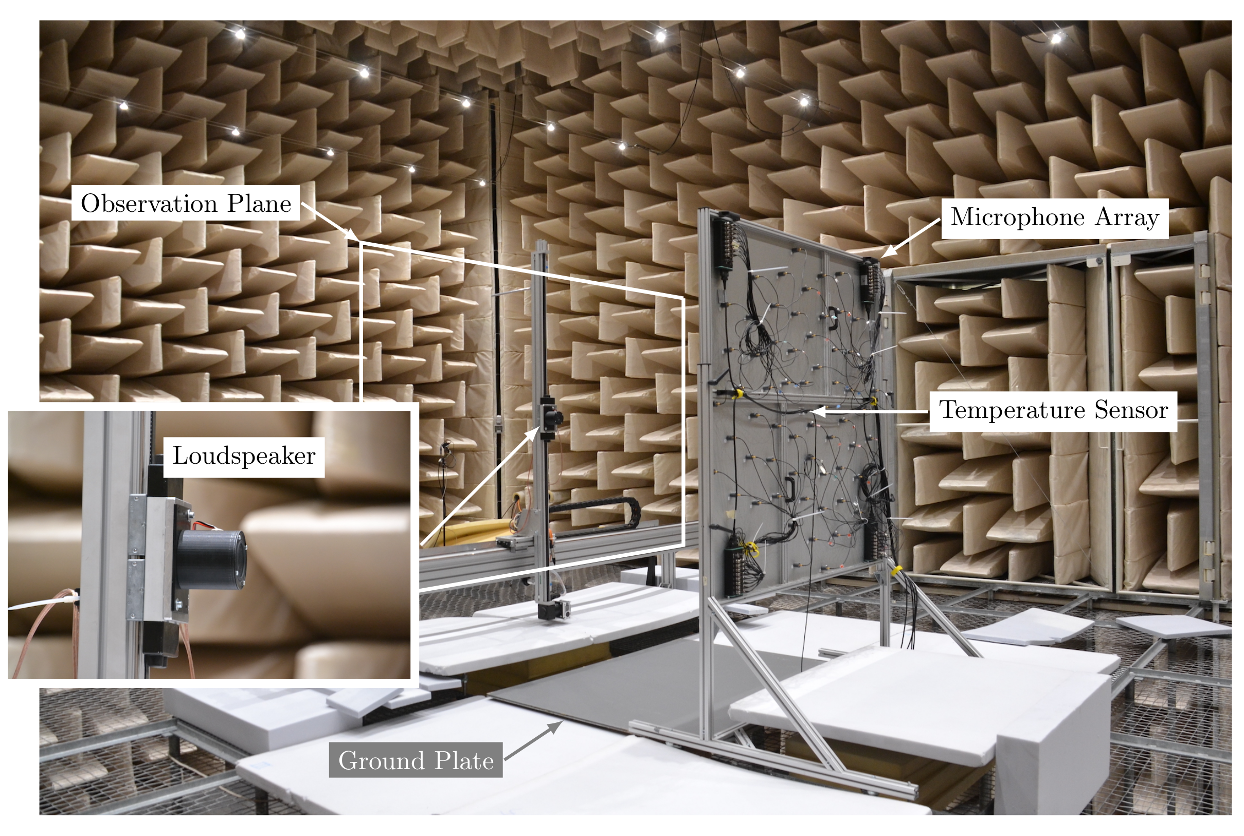
Measurement setup R2 from the MIRACLE dataset (reflective ground plate).

What the MIRACLE SRIRs represent

The MIRACLE dataset provides large-scale SRIR measurements acquired with a planar 64-channel array (Vogel spiral, aperture 1.47 m) in the anechoic chamber of TU Berlin. A reflective environment is realized in one scenario by inserting a ground plate between source and array.

In addition to SRIRs, MIRACLE provides metadata relevant for learning and benchmarking, including experimentally obtained loudspeaker directivity information and validated/offset- corrected source positions.

Scenarios

MIRACLE provides SRIRs for four measurement scenarios. In AcouPipe, the scenario is selected via the scenario parameter of DatasetMIRACLE.

The table below summarizes the spatial sampling and environmental configuration. Note that the number of available single-channel SRIRs per scenario is given by (# sources) × (64 microphones), and the full dataset comprises 856,128 single-channel impulse responses across all scenarios.

Available MIRACLE scenarios (SRIR grids and meta-data)

Scenario	Environment	c0	# sources	dx = dy	dz	Δx = Δy	Notes
A1	Anechoic	344.8 m/s	64 × 64 = 4096	146.7 cm	73.4 cm	23.3 mm	short distance
D1	Anechoic	345.0 m/s	33 × 33 = 1089	16.0 cm	73.4 cm	5.0 mm	dense local grid
A2	Anechoic	345.3 m/s	64 × 64 = 4096	146.7 cm	146.7 cm	23.3 mm	long distance
R2	Reflective ground plate	345.4 m/s	64 × 64 = 4096	146.7 cm	146.7 cm	23.3 mm	specular reflection

Default FFT parameters

The underlying default FFT parameters are:

FFT Parameters

Sampling Rate	fs = 32,000 Hz
Block size	256 samples
Block overlap	50 %
Windowing	von Hann / Hanning

Note

The FFT settings relate to feature extraction (e.g., CSM / beamforming) and can be overridden in your generation pipeline if required.

Randomized properties

Several properties of the dataset are randomized for each source case when generating data. This includes the number of sources, their positions, and their strengths. By default, source positions are sampled from the discrete source grid of the selected MIRACLE scenario.

Randomized properties (defaults)

No. of sources	Poisson distributed (\(\lambda = 3\))
Source positions	Bivariate normal distributed (\(\sigma = 0.1688 d_a\))
Source strength (\([{Pa}^2]\) at reference position)	Rayleigh distributed (\(\sigma_R = 5\))
Relative noise variance	Uniform distributed (\(10^{-6}\), \(0.1\))

Example

The following example script generates sourcemaps for several MIRACLE scenarios and is also used to create the figure below.

Example usage of DatasetMIRACLE

from pathlib import Path

import acoular as ac
import matplotlib.pyplot as plt

from acoupipe.datasets.experimental import DatasetMIRACLE

f = 2000

fig, axs = plt.subplots(1, 3, figsize=(9, 3), sharey=True, sharex=True)
fig.suptitle(f"Sourcemap ($f={f}$ Hz)", fontsize=12)

for i, scenario in enumerate([ "A1", "A2", "R2"]):

    dataset = DatasetMIRACLE(scenario=scenario, mode="wishart")
    data_generator = dataset.generate(
        features=["sourcemap", "loc", "f"],
        split="training",
        size=1,
        f=[f],
        num=0,
    )
    data_sample = next(data_generator)

    extent = dataset.config.grid.extent

    # sound pressure level
    Lm = ac.L_p(data_sample["sourcemap"]).T
    if i == 0:
        Lm_max = Lm.max()
        Lm_min = Lm.max() - 20

    axs[i].set_title(f"scenario: {scenario}")
    im = axs[i].imshow(Lm, vmax=Lm_max, vmin=Lm_min, extent=extent, origin="lower",interpolation="bicubic")

    # plot source locations
    for loc in data_sample["loc"].T:
        axs[i].scatter(loc[0], loc[1], s=1)
    axs[i].set_xlabel("x (m)")
    axs[i].set_ylabel("y (m)")

fig.colorbar(im, label="Sound Pressure Level (dB)", ax=axs[i])
fig.tight_layout()

The generator yields one sample at a time as a dictionary, including helper fields idx and seeds to keep data generation reproducible when running in parallel.

Example sourcemaps

License and access

MIRACLE is distributed under CC BY-NC-SA 4.0 (non-commercial). Please ensure your intended use complies with the license terms.